A fundamental principle in problem-solving is to try to break it down into smaller parts that may be easier to tackle. This concept also applies to programming. Our algorithms can be decomposed into subalgorithms that solve a smaller aspect of the problem. This process is known as algorithmic decomposition or modular decomposition. Each subalgorithm should be independent of the others and can be further decomposed into simpler parts in what is known as successive refinement. If a program is too long, it runs the risk of being difficult to understand as a whole, but it can always be divided into simpler and more manageable sections. A subalgorithm is written once and then used by all algorithms that need it.
When an algorithm requests that the actions established by a subalgorithm be performed, we say it is being called or invoked. The algorithm that invokes subalgorithms is sometimes called the main algorithm to emphasize the idea that, from the main course of action, the execution of some tasks is occasionally delegated to the subalgorithm.
The use of subalgorithms, by separately developing certain parts of the problem, is particularly advantageous in the following cases:
In complex algorithms: If the algorithm, and subsequently the program, is written continuously and in a single code file, it becomes very difficult to understand because the overall structure is lost due to the large number of operations it comprises. By isolating certain parts as separate subalgorithms, complexity is reduced.
When similar operations are repeated: If solving a problem requires performing a task that is repeated several times in the algorithm, we can define that task as a separate subalgorithm. This way, its code will be written only once, even if it is used in many parts of the program.
In the world of programming, there are many terms to define different types of subalgorithms: subroutines, functions, procedures, methods, subprograms, etc. It is not possible to obtain a definition that captures all the variants that exist in the use of these terms because the meaning of each of them often varies depending on the programming paradigm1 and the chosen programming language. What each of them means depends on the programming paradigm used and the chosen language, so there is no definition that is general enough for each one.
Throughout this tutorial, and while using R, we will refer to subalgorithms as functions, and for now, we will use them to help with program modularity.
Turning right
To start with something simple, in the example seen in the previous
section, Karel needed to turn right, and we achieved that by telling it
to turn left three times. This is a bit inconvenient, firstly because
mentally we imagine something else when we want Karel to turn right, and
secondly because Karel will probably need to turn right in many
problems, and we won’t want to repeat
turn_left() so many times.
That’s why it’s very reasonable to create a new function to handle this. Every time we realize that we are using a sequence of Karel commands to accomplish a specific task, such as turning right, it is time to define a new function that encompasses those commands:
In general, in R, a function is created following these steps:
- Choose a name:
girar_derecha(turn_right). - Use the assignment operator (or arrow,
<-) to associate the function definition with that name. - Write the instruction
function() {...}, where the actions encompassed by the new function are placed inside the curly braces, one action per line:
Using this subalgorithm, we can see how the code writing is
simplified. It is important to note that for us to be able to use the
turn_left() function, it has to be defined
by the user and evaluated by R before we want to use it
to solve our problem:
# --------------- Load Karel package --------------------
library(karel)
# ------------ Definition of auxiliary functions -----------
turn_right <- function() {
  turn_left()
  turn_left()
  turn_left()
}
# ---------------- Main programa ----------------------
generate_world("mundo001")
move()
pick_beeper()
move()
turn_left()
move()
put_beeper()
move()
move()
put_beeper()
move()
run_actions()
EXERCISE: Create a function called
turn_around() that allows Karel to make a
180-degree turn and face the opposite direction.
Karel’s superpowers
In the previous section, we created the
turn_right() and
turn_around() functions on our own to
learn how to generate new subalgorithms. However, to streamline the
creation of our programs and the visualization of Karel’s actions, the R
package provides enhanced versions of
turn_right() and
turn_around(). To make them available for
use, we need to activate Karel’s superpowers with the following
statement, which can be executed at any time (after
library(karel) would be a good place):
Filling the hole
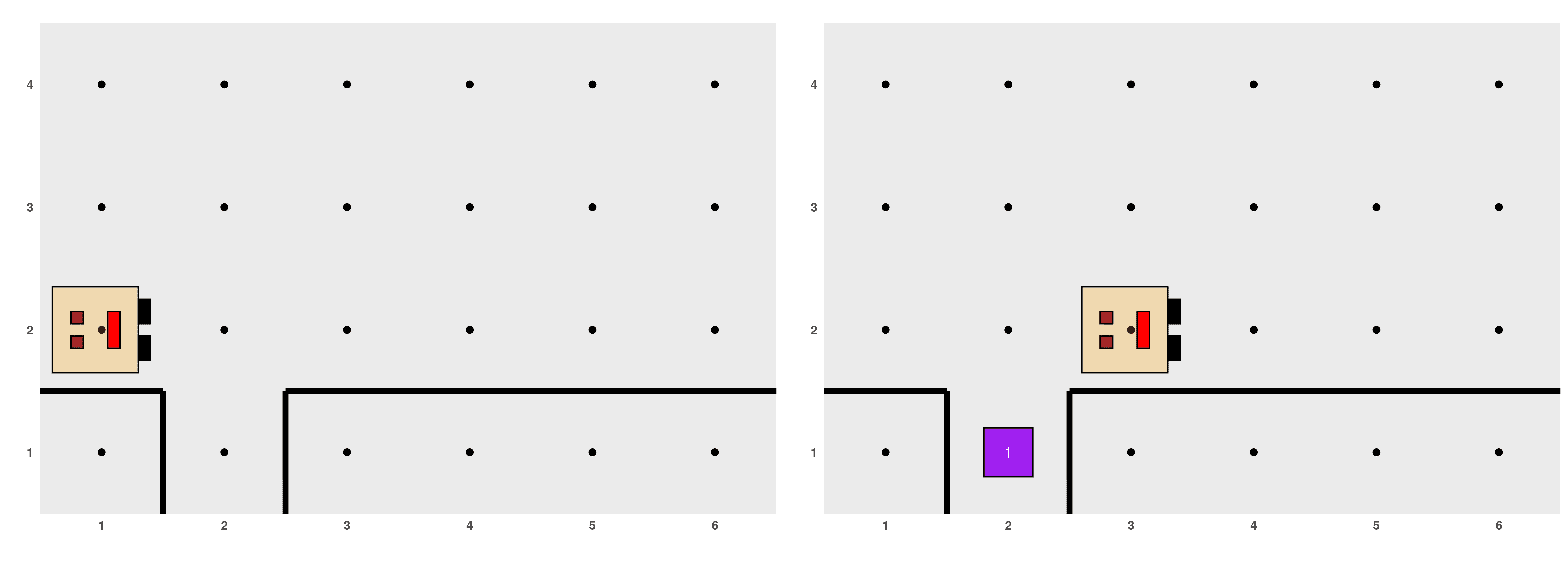
Let’s see another example of the usefulness of algorithmic decomposition. As it happens in many places, in Karel’s world, streets sometimes need repair. Let’s imagine Karel is walking down the street as shown in the left figure and encounters a hole. The task is to fill it with a beeper and move to the other end, as shown in the right figure.
If we limit ourselves to Karel’s basic commands, the program to solve this is:
generate_world("mundo002")
move()
turn_left()
turn_left()
turn_left()
move()
put_beeper()
turn_left()
turn_left()
move()
turn_left()
turn_left()
turn_left()
move()
run_actions()However, if we use our own functions
turn_right() and
turn_around(), the program becomes shorter
and clearer:
generate_world("mundo002")
move()
turn_right()
move()
put_beeper()
turn_around()
move()
turn_right()
move()
run_actions()Now, filling the hole can be seen as a specific task that can be thought of as a problem in itself, which can be solved separately from the main algorithm. We can define a new subalgorithm specifically for this task, which can be reused in other situations. Following the idea of algorithmic decomposition, the problem we are analyzing can be decomposed as follows:
# --------------- Load Karel package --------------------
library(karel)
load_super_karel() # makes turn_right() and turn_around() available
# ------------ Definition of auxiliary functions -----------
fill_hole <- function() {
turn_right()
move()
put_beeper()
turn_around()
move()
turn_right()
}
# ------------------- Main program --------------------
generate_world("mundo002")
move()
fill_hole()
move()
run_actions()
Documentation of subalgorithms
In the context of programming, documentation means writing instructions so that other people can understand what we want to do in our code or how to use our functions. For example, as we saw earlier, all predefined R functions are documented so that we can seek help if needed. When creating our own subalgorithms, it is important to include comments to guide other people (and ourselves in the future if we forget) on what and how we are developing. For example, it may be good to state the name of the function and clarify under what initial condition it can be used and what final result it produces, for example:
#  --------------- Load Karel package --------------------

library(karel)
load_super_karel()

# ------------ Definition of auxiliary functions -----------

# Function: fill_hole
# Initial condition: Karel is on top of the hole (on the previous street),
# facing east
# Final condition: Karel is in the same position as at the beginning and has
# placed a beeper in the hole
fill_hole <- function() {
  turn_right()
  move()
  put_beeper()
  turn_around()
  move()
  turn_right()
}

# ------------------- Main program -------------------
generate_world("mundo002")
move()
fill_hole()
move()
run_actions()
Some examples presented in this tutorial were adapted from “Karel the Robot Learns Java” by Eric Roberts, published in 2005.